|
Overview
|
|
Image Analysis
-
Introduction
Image analysis involves manipulating the image data to determine
exactly the information necessary to help solve a computer imaging
problem. The image analysis process, can be divided into three primary
stages: 1) Preprocessing, 2) Data Reduction and 3) Feature Analysis.
-
Preprocessing:
It is used to remove noise and eliminate irrelevant, visually
unnecessary information.
-
Data Reduction:
It involves either reducing the data in the spatial domain or
transforming it into another domain called the frequency domain and
then extracting features for the analysis process.
-
Feature Analysis:
In this the features extracted by the data reduction process are
examined and evaluated for their use in the application.
After the analysis we have a feedback loop that provides for an
application-specific review of the analysis results.
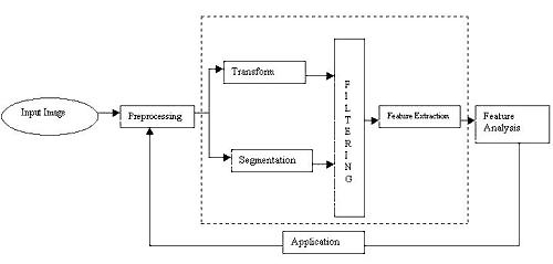 Image Analysis - System Model
|
|
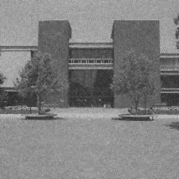
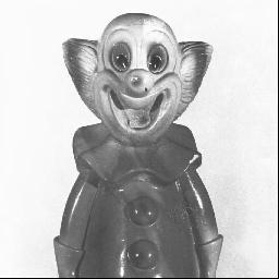
Segmentation & Morphological Filtering
Image segmentation is used to find regions that represent objects or
meaningful parts of objects. Image segmentation methods will look for
objects that either have some measure of homogeneity within themselves
or have some measures of contrast with objects on their border.
Gray level morphology relates to the structure or form of objects in a
gray-level image. Morphological filtering simplifies a segmented image to
facilitate the search for objects of interest. This is done by smoothing
out object outlines, filling small holes, eliminating small projections.
The basic morphological operations are Dilation, Erosion, Opening and
Closing.
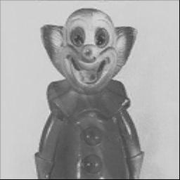
 Original image Original image
|
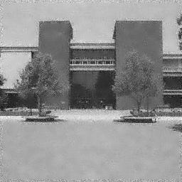
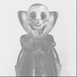
 Image after morphological opening Image after morphological opening
|
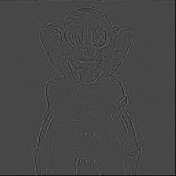
 Image after morphological closing Image after morphological closing
|
|
|
|
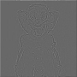
Fourier Transform
The Fourier transform uses sinusoidal functions as basis functions. The
magnitude of the fourier spectrum can be displayed as an image. Normaly
the magnitude is log-remapped for display, otherwise all that is seen is
the DC term.
 Original image Original image
|
 Fourier transform linearly remapped Fourier transform linearly remapped
|
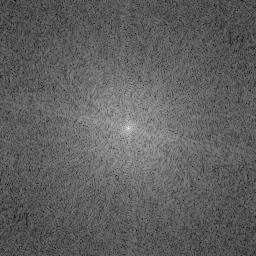 Fourier transform log remapped Fourier transform log remapped
|
|
|
|
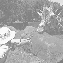
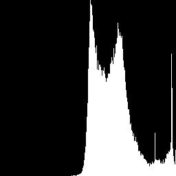
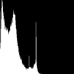
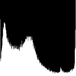
Histogram Features
The Histogram of an image is a plot of the gray-level values versus the
number of pixels at that value. The shape of the histogram provides us
with information about the nature of the image , or subimage if we are
considering an object within image.
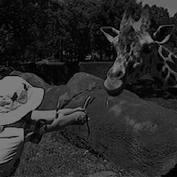
 Bright Image Bright Image
|
 Histogram appears shifted to the right Histogram appears shifted to the right
|
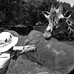
 Dark Image Dark Image
|
 Histogram appears shifted to the left Histogram appears shifted to the left
|
 High-contrast Image High-contrast Image
|
 Histogram appears spread out Histogram appears spread out
|
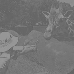 Low-contrast image Low-contrast image
|
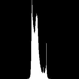 Histogram appears clustered Histogram appears clustered
|
|
|
Image Restoration
Image restoration methods are used to improve the appearance of an image
by application of a restoration process that uses a mathematical model for
image degradation.
In this, degraded images and knowledge of the image creation process are
provided as input to the development of the degradation model. After the
degradation process has been developed, the formulation of the inverse
process follows. This inverse degradation process is then applied to the
degraded image, d(r,c), which results in the output image I(r,c). This
output image I(r,c) is the restored image that represents an estimate of
the original image I(r,c).
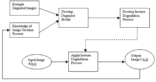 Image Restoration -System Model
|
|
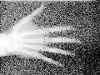
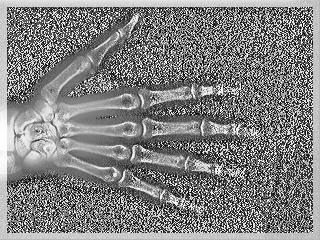
Adaptive Filter
An adaptive filter alters its basic behavior as the image is processed. It
may act like a mean filter on some parts of the image and as a median
filter on other parts of the image. The minimum mean-square error (MMSE)
filter is a good example of an adaptive filter, which exhibits varying
behavior based on local image statistics.The MMSE filter works best with
gaussian or uniform noise.
 a. Original image a. Original image
|
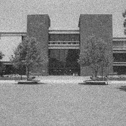 b. Image with gaussian noise-variance=300; mean=0 b. Image with gaussian noise-variance=300; mean=0
|
 c. Result of MMSE filter --kernel size=3; noise variance=300 c. Result of MMSE filter --kernel size=3; noise variance=300
|
 d. Result of MMSE filter--kernel size=9; noise variance =300 d. Result of MMSE filter--kernel size=9; noise variance =300
|
|
|
Geometric Transform
Geometric transforms are used to modify the location of pixel values
within an image, typically to correct images that have been spatially
distorted. These methods are often referred to as rubber-sheet transforms
because the image is modeled as a sheet of rubber and stretched and shrunk,
or otherwise manipulated, as required to correct for any spatial
distortion. It requires two steps 1) Spatial Transform and 2) Gray-Level
Interpolation.
-
Spatial Transform:
Spatial transforms are used to map the input image location to a
location in the output image; it defines how the pixel values in
the output image are to be arranged. The method to restore a
geometrically distorted image consists of three steps: 1) define
quadrilaterals (four-sided polygons) with known or best-guessed
tiepoints for the entire image, 2) find the equations R(r,c) and
C(r,c) for each set of tiepoints, and 3) remap all the pixels
within each quadrilateral subimage using the equations
corresponding to those tiepoints.
-
Gray-Level Interpolation:
The simplest method of gray-level interpolation is the nearest
neighbor method.Where the pixel is assigned the value of the closest
pixel in the distorted image.This method does not necessarily provide
optimal results but has the advantage of being easy to implement and
computationally fast.
 Original image Original image
|
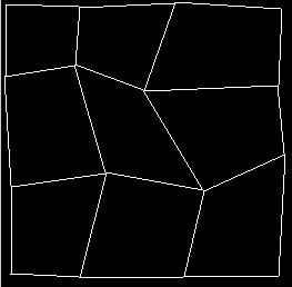 A mesh defined by 16 tiepoints will be used to first distort and then restore the image. A mesh defined by 16 tiepoints will be used to first distort and then restore the image.
|
 The original image has been distorted using the bilinear interpolation method. The original image has been distorted using the bilinear interpolation method.
|
 Restoration by the nearest neighbor method shows the blocky effect that occurs at edges. Restoration by the nearest neighbor method shows the blocky effect that occurs at edges.
|
 Restoration with neighborhood averaging interpolation provides smoother edges than with the nearest neighbor method, but it also blurs the image. Restoration with neighborhood averaging interpolation provides smoother edges than with the nearest neighbor method, but it also blurs the image.
|
 Restoration by bilinear interpolation provides optimal results. Note that some distortion occurs at the boundaries of the mesh quadrilaterals. Restoration by bilinear interpolation provides optimal results. Note that some distortion occurs at the boundaries of the mesh quadrilaterals.
|
|
|
Image Enhancement
Image enhancement techniques are used to emphasize and sharpen image
features for display and analysis. Enhancement methods operate in the
spatial domain by manipulating the pixel data or in the frequency domain
by modifying the spectral components. The type of techniques include:
-
Point operation:
Here each pixel is modified according to a particular equation that is
not dependent on other pixel values.
-
Mask operation:
Here each pixel is modified according to the values of the pixel's
neighbors.
-
Global operation:
Here all the pixel values in the image ( or subimage) are taken into
consideration.
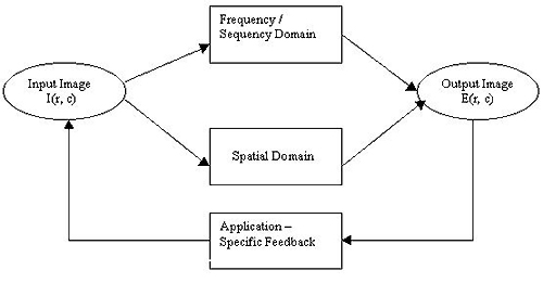 Image Enhancement- System Model
|
|
Adaptive Contrast Enhancement
Adaptive contrast enhancement refers to modification of gray-level values
within an image based on some criterion that adjusts its parameters as a
local image characteristics change. The adaptive contrast enhancement
filter is used with an image which has uneven contrast, where we want to
adjust the contrast differently in different regions of the image. It
works by using both local and global image statistics to determine regions
of the image.
Original image
|
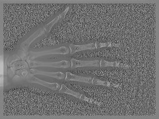
Image after using ACE filter
|
Histogram equalization of original Image
|
Histogram equalization of Image after using ACE filter
|
|
|
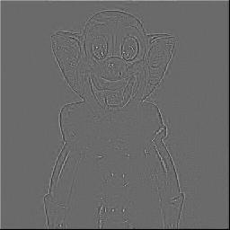
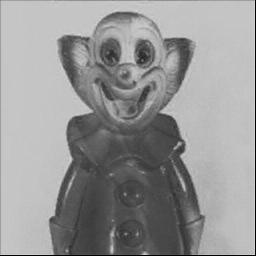
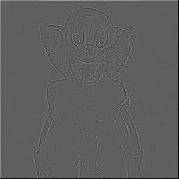
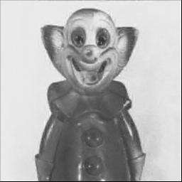
Unsharp Masking
Unsharp masking enhancement algorithm is representative of practical image
sharpening methods. It combines many operations like filtering and
histogram modifications.
 Original image Original image
|
 Unsharp masking with lower limit=0, upper=100, with 2% low and high clipping Unsharp masking with lower limit=0, upper=100, with 2% low and high clipping
|
 Original Image Unsharp masking with lower limit=0, upper=150, with 2% low and high clipping Original Image Unsharp masking with lower limit=0, upper=150, with 2% low and high clipping
|
 Image Unsharp masking with lower limit=0, upper=200, with 2% low and high clipping Image Unsharp masking with lower limit=0, upper=200, with 2% low and high clipping
|
|
|
Image Compression
Image compression involves reducing the size of image data files, while
retaining necessary information. The resulting file is called the
compressed file and is used to reconstruct the image, resulting in the
decompressed image.
The compression system model consists of two parts: the Compressor and
the Decompressor.
-
Compressor:
It consists of a preprocessing stage and encoding stage. The first
stage in preprocessing is data reduction. For example, the image data
can be reduced by gray level and/or spatial quantization. The second
step in preprocessing is the mapping process, which maps the original
image data in to another mathematical space, where it is easier to
compress the data. Next, as part of the encoding process, is the
quantization stage, which takes the potentially continuous data from
the mapping stage and puts it in discrete form. The final stage of
encoding involves the coding the resulting data, which maps the
discrete data from the quantizer onto a code in an optimal manner.
-
Decompressor:
In this the decoding process is divided into two stages.First, it
takes the compressed file and reverses the original coding by mapping
the codes to the original, quantized values.Next, these values are
processed by a stage that performs an inverse mapping to reverse the
original mapping process. Finally, the image may be postprocessed to
enhance the look of the final image.
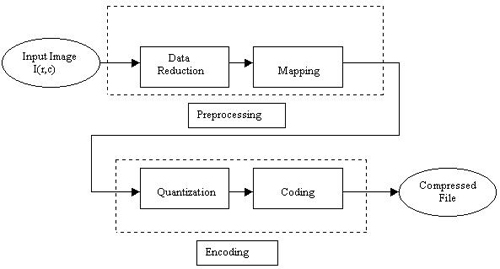 Compressor- System Model
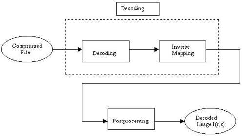 Decompressor - System Model
|
|
Wavelet/Vector Quantization
The Wavelet-based compression shows much promise for the next generation
of image compression methods. Because wavelets localize information in
both the spatial and frequency domains, we consider these to be hybrid
methods. The wavelet transform combined with vector quantization has led
to the development of compression algorithms with high compression ratios.
 a. Original image a. Original image
|
|
 b. WVQ compression ratio 10:1 b. WVQ compression ratio 10:1
|
 c. Error of image (b) c. Error of image (b)
|
 d. WVQ compression ratio 15:1 d. WVQ compression ratio 15:1
|
 e. Error of image (d) e. Error of image (d)
|
 f. WVQ compression ratio 33:1 f. WVQ compression ratio 33:1
|
 g. Error of image (f) g. Error of image (f)
|
 h. WVQ compression ratio 36:1 h. WVQ compression ratio 36:1
|
 i. Error of image (h) i. Error of image (h)
|
|
|
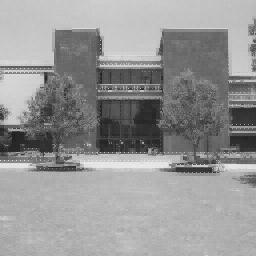
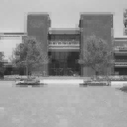
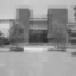
Block Truncation Coding
Block truncation coding is a type of lossy compression which works by
dividing the image into small subimages and then reducing the number of
gray levels in each block. This reduction is performed by a quantizer that
adapts to the local image statistics. The levels for quantizer are chosen
to minimize a specified error criterion, and then all the pixel values
within each block are mapped to quantized levels.
 Original Image having 65536 bytes. Original Image having 65536 bytes.
|
 Original Image having 65536 bytes. Compressed data occupies 16419 bytes. Compression ratio 1:4 Original Image having 65536 bytes. Compressed data occupies 16419 bytes. Compression ratio 1:4
|
 Original Image having 65536 bytes. Compressed data occupies 8739 bytes. Compression ratio is 1:8. Original Image having 65536 bytes. Compressed data occupies 8739 bytes. Compression ratio is 1:8.
|
 Original Image having 65536 bytes. Compressed data occupies 3142bytes. Compression ratio is 1:15. Original Image having 65536 bytes. Compressed data occupies 3142bytes. Compression ratio is 1:15.
|
|
|
|